Potential Field Navigation: Obstacle definition in Python using a Gaussian Field

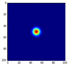
First let’s start with some basic assumptions.  We define a 2D environment of size x_max, y_max. We can easily represent this environment in Python as a Grid of size (x_max, y_max). The resolution of this Grid is not important for now, since later it is possible to convert Grid values to meters for example.  We want to simulate an obstacle in a particular position of this environment, let’s say that the obstacle position will be p_obs = (x_obs, y_obs) and that the complete shape of this obstacle can be fitted inside a circle of radius = 10 grid units.

One way of representing this obstacle for potential field navigation is by using a Gaussian repulsor field in the center of the obstacle. The following code creates a Grid and then calculates the potential field for the given obstacle position.

def gaussian_obstacle(X,Y, x_obs, y_obs, size_robot, size_obstacle):
    #We extend the size of the obstacle with the size of the robot (border expansion)
    ext_size = size_robot + size_obstacle
    sigma_x = (ext_size/2)/2.3548
    sigma_y = (ext_size/2)/2.3548
    theta = 0
    A = 100 #Weight of the Gaussian
    Z = zeros_like(X)
    a = cos(theta)**2/2/sigma_x**2 + sin(theta)**2/2/sigma_y**2
    b = -sin(2*theta)/4/sigma_x**2 + sin(2*theta)/4/sigma_y**2
    c = sin(theta)**2/2/sigma_x**2 + cos(theta)**2/2/sigma_y**2
    Z[:] = Z[:]+A*exp( - (a*(X-x_obs)**2 + 2*b*(X-x_obs)*(Y-y_obs) + c*(Y-y_obs)**2))
    return Z

Z = gaussian_obstacle(X, Y, 50, 50, 10, 10)

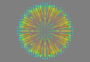
We then create a gradient field based on the scalar field:

def calculate_vector_field(Z):
    U, V = gradient(Z,1,1)
    U = -U
    V = -V
    return U, V

U, V = calculate_vector_field(Z)

Which will produce this vectors centered in the position of the obstacle

 

Finally to obtain a vector reference (velocity) for a robot that is currently at position (41,41), you may use the following function:

def get_velocity_command(U, V, x_robot, y_robot):
return U[x_robot,y_robot], V[x_robot,y_robot]

Vx_robot, Vy_robot = get_velocity_command(U, V, 41, 41)

If you have many moving obstacles and a big environment it may be too computationally expensive to do the calculation for the whole Grid, a possible solution is to do the calculation only in the surrounding area of the robot and obtain only the reference vector for the current position of the robot:

p_robot = (rob_x, rob_y)
#We create a minimal grid around the position of our robot
X, Y = mgrid[(rob_x-1):(rob_x+1)+1,(rob_y-1):(rob_y+1)+1]

Complete code with plots using Mayavi from enthought.

from pylab import *
import matplotlib.pyplot as plt
from mayavi import mlab

x_min = 0
y_min = 0
x_max = 100
y_max = 100
X, Y = mgrid[ x_min:x_max+1:1,  y_min: y_max+1:1]

def gaussian_obstacle(X,Y, x_obs, y_obs, size_robot, size_obstacle):
    #We extend the size of the obstacle with the size of the robot (border expansion)
    ext_size = size_robot + size_obstacle
    sigma_x = (ext_size/2)/2.3548
    sigma_y = (ext_size/2)/2.3548
    theta = 0
    A = 100 #Weight of the Gaussian
    Z = zeros_like(X)
    a = cos(theta)**2/2/sigma_x**2 + sin(theta)**2/2/sigma_y**2
    b = -sin(2*theta)/4/sigma_x**2 + sin(2*theta)/4/sigma_y**2
    c = sin(theta)**2/2/sigma_x**2 + cos(theta)**2/2/sigma_y**2
    Z[:] = Z[:]+A*exp( - (a*(X-x_obs)**2 + 2*b*(X-x_obs)*(Y-y_obs) + c*(Y-y_obs)**2))
    return Z

def calculate_vector_field(Z):
    U, V = gradient(Z,1,1)
    U = -U
    V = -V
    return U, V

Z = gaussian_obstacle(X, Y, 50, 50, 10, 10)
U, V = calculate_vector_field(Z)


def get_velocity_command(U, V, x_robot, y_robot):
    return U[x_robot,y_robot], V[x_robot,y_robot]
    
Vx_robot, Vy_robot = get_velocity_command(U, V, 40, 40)

# Plot
mlab.figure(size=(800, 600))
mlab.quiver3d(X, Y, zeros_like(X), U, V,zeros_like(U))
mlab.mesh(X, Y, Z)
mlab.show()